Finite Element Method Magnetics

Magnetostatics

• FEMM 4.2 Magnetics, Electrostatics, Heat Flow, and Current Flow

http://www.femm.info/wiki/HomePage

• Wiki. Magnetostatics

https://en.wikipedia.org/wiki/Magnetostatics

• Permanent Magnet Example

http://www.femm.info/wiki/PermanentMagnetExample

• Magnetostatic Tutorial

http://www.femm.info/wiki/MagneticsTutorial

• How to make magnet

A BH Curve describes the magnetic properties of the magnetic material.  Let’s examine one step by step.

---

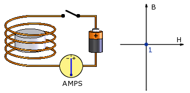
Consider a neodymium magnet sitting inside a magnetizer.  The magnetizer is essentially a coil of wire wrapped around the magnet, through which we will apply a very strong current to create a magnetic field.

In the graph at right, the horizontal axis shows the strength of the Applied magnetic field (H) – the one we get by running current through the wire.  The vertical axis shows the Induced field (B), which the permanent magnet creates by itself.

The magnet we will start with has just been manufactured, but not yet magnetized.  The magnetic field it creates is zero (B).  There is no current running through the wire, so the applied field (H) is also zero.  Let’s represent this point with a dot at the zero location on the graph, point #1.

---

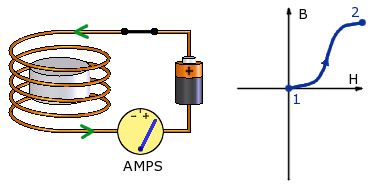
Now, let’s briefly run a terrifically strong current through the wire, placing the magnet in a uniform magnetic field.  Keep increasing the current, and the applied field increases.  If we measure the magnetic field, we also see an induced magnetic field, made from the magnet.

At point #2, the increases level off.  At point #2, we still have a current running through the wire producing an Applied field, plus an Induced field from the magnet.

---

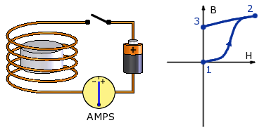
Now, let’s turn the current off.  The Applied field (H) drops to zero, but there remains a magnetic field produced by the magnet, shown as point #3. This point is also called Br, Br max, the Residual Induction or the Residual Flux Density.

In our Glossary, we define Br as, “the magnetic induction remaining in a saturated magnetic material after the magnetizing field has been removed.”  That's at point #3.

---

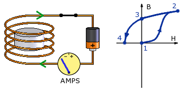
If we apply a current in the opposite direction, the magnetic field created by the current in the coil of wire opposes the field from the magnet -- it is in the opposite direction.

By applying progressively more current in this direction, we can find the shape of the normal curve in the second quadrant (the upper left hand quarter) of the BH Curve graph.  Where the Induced field reaches zero, at point #4, is called the Coercive force, Hc.  This is the magnet's Coercivity: the measure of the magnet’s resistance to demagnetization by an external magnetic field.

The farther left on the graph this point is located, the stronger the magnetic field you need to demagnetize the magnet.  Not only are neodymium magnets strong, but they have the highest coercivity values of all permanent magnet types.

---

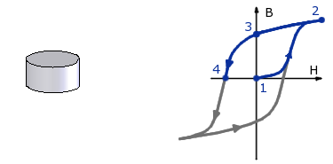
The rest of the graph follows a symmetric form.  The whole shape of this graph is the hysteresis curve, and defines how a particular magnet material behaves. It is a property of the magnet material.

When considering the performance of an already magnetized magnet in an application, we only need to look at the 2^nd quadrant (the upper left quarter of the graph) to see how it will behave.